From Lines to Planes: Understanding Two-Dimensional Linear Systems
Breaking Free from the Line
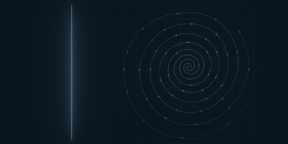
After spending chapters confined to one-dimensional flows, stepping into two dimensions feels like breaking free from a cage.
On a line, trajectories move monotonically or stay put — they have nowhere else to go.
But on a plane, trajectories can swirl, spiral, and orbit, revealing rich behaviors impossible in one dimension.
What Are Linear Systems?
A two-dimensional linear system has the form:
In matrix form:
Because linear systems satisfy superposition, if
The origin
The Phase Plane
Solutions now evolve on the
Each point
The path traced by a solution is called a trajectory, and the full collection is the phase portrait.
The Simple Harmonic Oscillator
For a mass–spring system:
Define
Vector Field Intuition
- On
-axis ( ): vectors point vertically — down for , up for . - On
-axis ( ): vectors point horizontally — right for , left for . - At the origin: zero vector → fixed point.
Closed Orbits = Oscillations
Trajectories form closed ellipses.
Physically:
- The mass oscillates periodically.
- Energy is conserved:
. - The origin is a center — neutrally stable.
Reading the Oscillation from the Orbit
- Maximum compression:
most negative, - Moving right:
increasing, - Passing equilibrium:
, max - Maximum extension:
most positive, - Moving left:
decreasing, - Back to start → repeats
Phase portraits turn dynamics into geometry.
Eigenvalues and Eigenvectors
We seek exponential solutions:
Substitute into
Thus
General Solution
If
The Six Basic Fixed-Point Types
1. Saddle Point (
- One stable, one unstable direction
- Stable manifold → eigenvector for
- Unstable manifold → eigenvector for
- Hyperbolic trajectories avoiding the origin
- Physically: balancing a pencil on its tip — unstable
2. Stable Node (
- Both eigenvalues negative → all trajectories approach the origin
- Tangent to the slow eigendirection
- Asymptotically stable
Special case:
3. Unstable Node (
Same geometry but reversed arrows — all trajectories diverge.
4. Stable Spiral (
- Spiral inward
- Decaying oscillations:
- Period
- Asymptotically stable
5. Unstable Spiral (
Spirals outward — oscillations grow with time.
6. Center (
- Purely imaginary eigenvalues
- Closed orbits
- Neutrally stable (Liapunov stable but not attracting)
The Classification Diagram
Let:
Eigenvalues:
Interpretation:
: saddle , : node , : spiral/center : stable : unstable : center
Stability Concepts
- Attracting: trajectories approach fixed point.
- Liapunov stable: trajectories stay close forever.
- Asymptotically stable: both attracting and Liapunov stable.
| Type | Stability |
|---|---|
| Nodes, spirals with | Asymptotically stable |
| Centers | Neutrally stable |
| Saddles, spirals with | Unstable |
A Delightful Application: Love Affairs
Let
Personality Types
| Parameters | Type |
|---|---|
| Eager beaver | |
| Cautious lover | |
| Narcissistic nerd | |
| Hermit |
Romeo echoes Juliet (
→ Center: endless cycles of love and hate!
Two cautious lovers:
with
- If
: stable node → apathy - If
: saddle → explosive passion
Moral: too much caution kills romance.
Quick Classification Steps
- Compute
, - If
: saddle - If
: non-isolated fixed points - Else check
: : node : star/degenerate : spiral or center
- Determine stability via
Why Linear Systems Matter
- Local Linearization: Near any fixed point of a nonlinear system, linearization via the Jacobian reveals local behavior.
- Pedagogical Value: Builds geometric intuition about phase space.
- Real-World Relevance: Many models (circuits, oscillators, epidemiology) are linear or locally linear.
Key Insights
- Geometry reveals dynamics.
- Eigenvalues and eigenvectors are geometric.
- Two numbers
classify everything. - Stability has layers: attracting vs Liapunov.
- Imaginary parts → rotation, real parts → decay/growth.
- Moving from 1D to 2D adds fundamentally new behavior.
Looking Ahead
- Nonlinear systems introduce limit cycles and chaos.
- Linearization remains the first step to understanding local behavior.
- The geometric mindset — thinking in terms of flows — is the essence of dynamical systems.
Mathematics isn’t just abstract — it can even explain why Romeo and Juliet’s love oscillated endlessly.
Their fate was sealed not only by family feuds, but by the eigenvalues of their emotional dynamics.
Reference
This post is based on material from Nonlinear Dynamics and Chaos by Steven H. Strogatz (1994).