
One-Dimensional Dynamical Systems
Introduction
Have you ever wondered how mathematicians predict the behavior of systems over time without solving complicated equations?
In my recent studies of dynamical systems, I discovered an elegant geometric approach that transforms differential equations into visual, intuitive flows. Let me share what I learned about one-dimensional systems and why they’re the perfect starting point for understanding dynamics.
What Are First-Order Systems?
A first-order (or one-dimensional) system is simply an equation of the form:
Here,
The dot notation (
These systems are called autonomous because they don’t depend explicitly on time—the rate of change at any point depends only on where you are, not when you are there.
The Power of Pictures Over Formulas
One of the most eye-opening lessons from this topic was that pictures often outperform formulas when analyzing nonlinear systems.
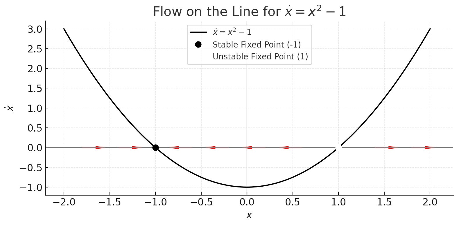
Consider the equation
- Plot
versus - Draw arrows on the x-axis showing the direction and speed of flow
- Immediately see where the system is heading
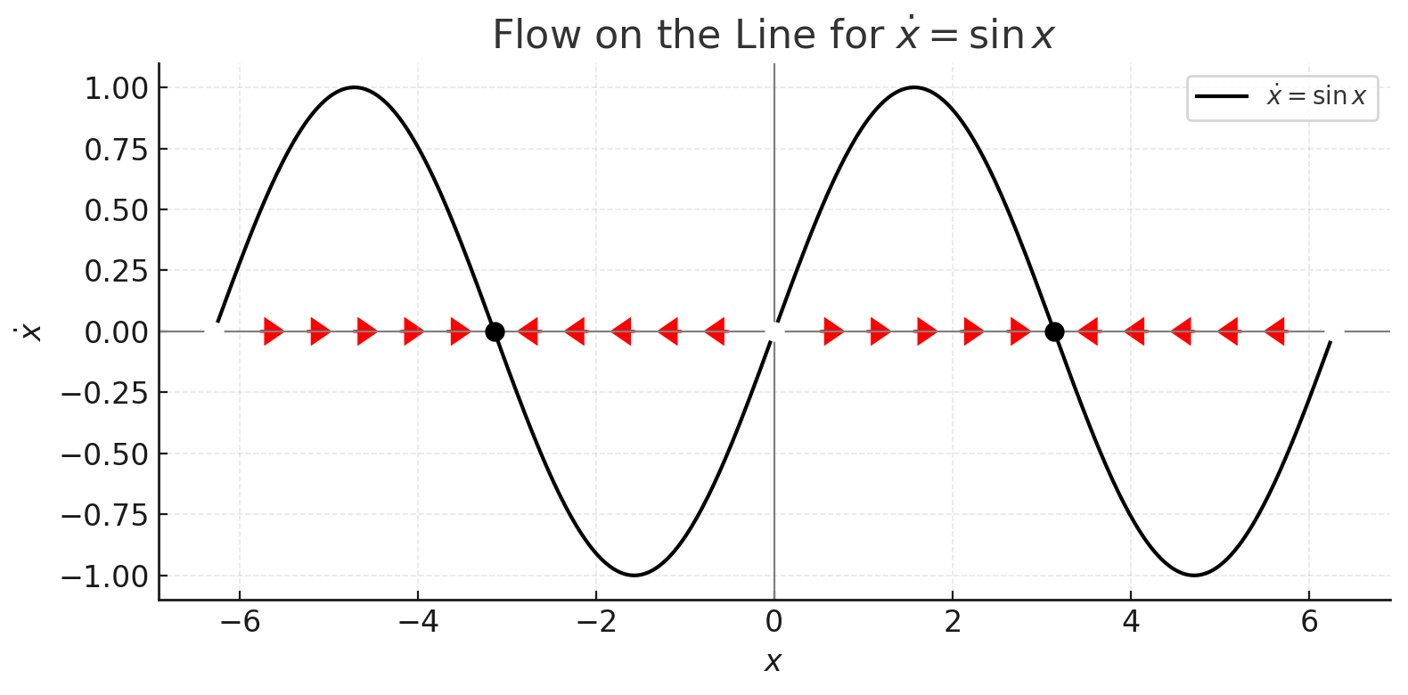
This visual approach reveals the system’s behavior at a glance, answering questions like “what happens as
The Vector Field Interpretation
Here’s the key insight: think of the differential equation as describing fluid flow along a line.
Imagine a river flowing along the real number line, where:
- The velocity at each point
is given by - Flow moves right when
- Flow moves left when
- Flow stops at points where
These stopping points are called fixed points or equilibrium points, and they’re the stars of the show in one-dimensional dynamics.
Fixed Points and Stability
Fixed points come in two flavors:
Stable Fixed Points (Attractors/Sinks)
- Represented by solid black dots
- The flow moves toward them from nearby points
- Small disturbances decay over time
- Think of a marble settling at the bottom of a bowl
Unstable Fixed Points (Repellers/Sources)
- Represented by open circles
- The flow moves away from them
- Small disturbances grow over time
- Think of a marble balanced on top of a hill
There’s also a rare third type called half-stable fixed points, which attract from one side and repel from the other.
A Real-World Example: The Logistic Equation
One of the most important applications is modeling population growth.
The simple exponential model
Where:
: population size : growth rate : carrying capacity (maximum sustainable population)
This model has two fixed points:
→ unstable (extinction is precarious) → stable (populations naturally approach carrying capacity)
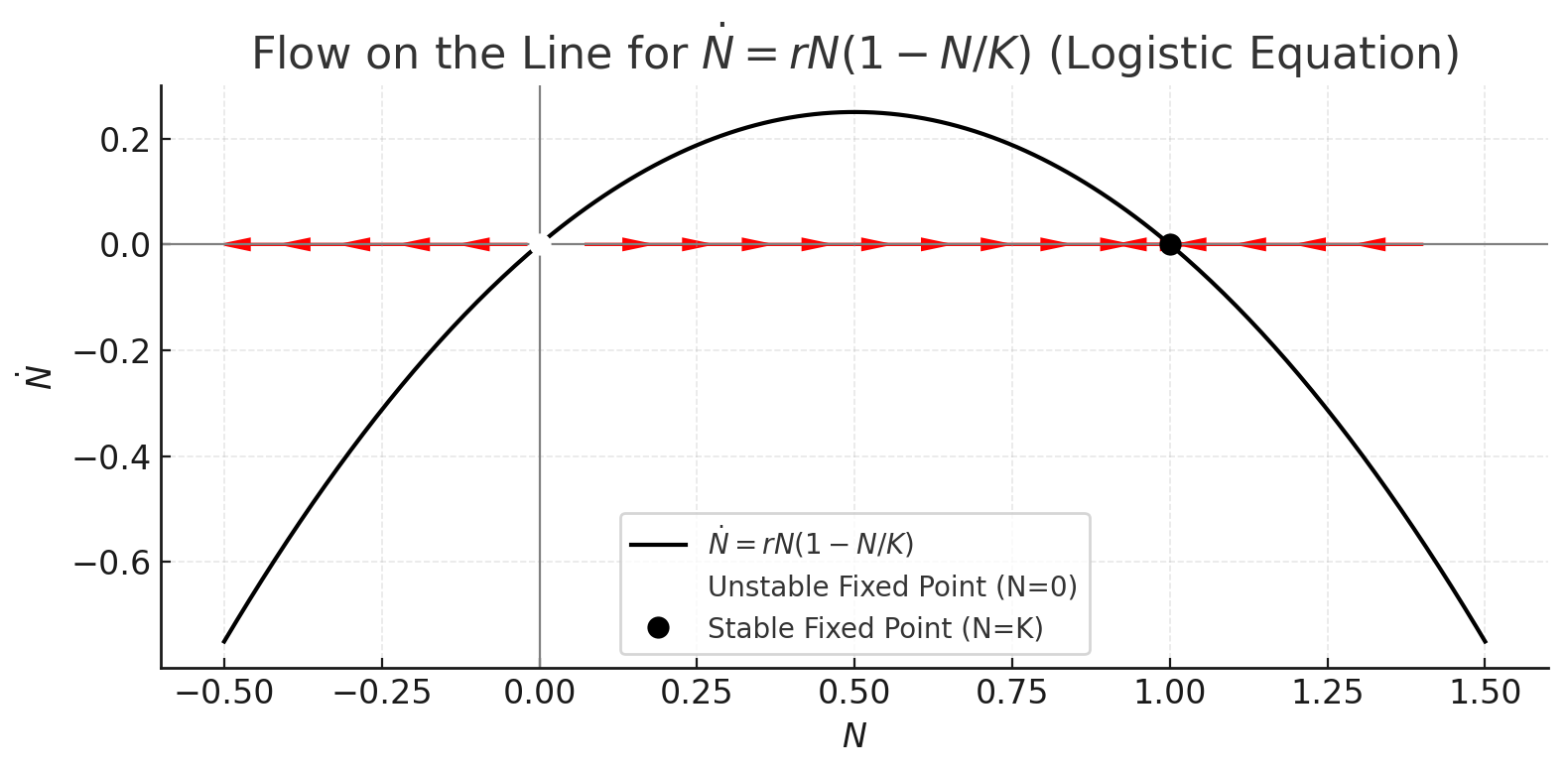
The phase portrait reveals that populations below
This captures the real-world behavior of resource-limited populations far better than exponential models.
How the Two Graphs Are Connected
The parabolic plot of
In the first graph,
When
Around
As
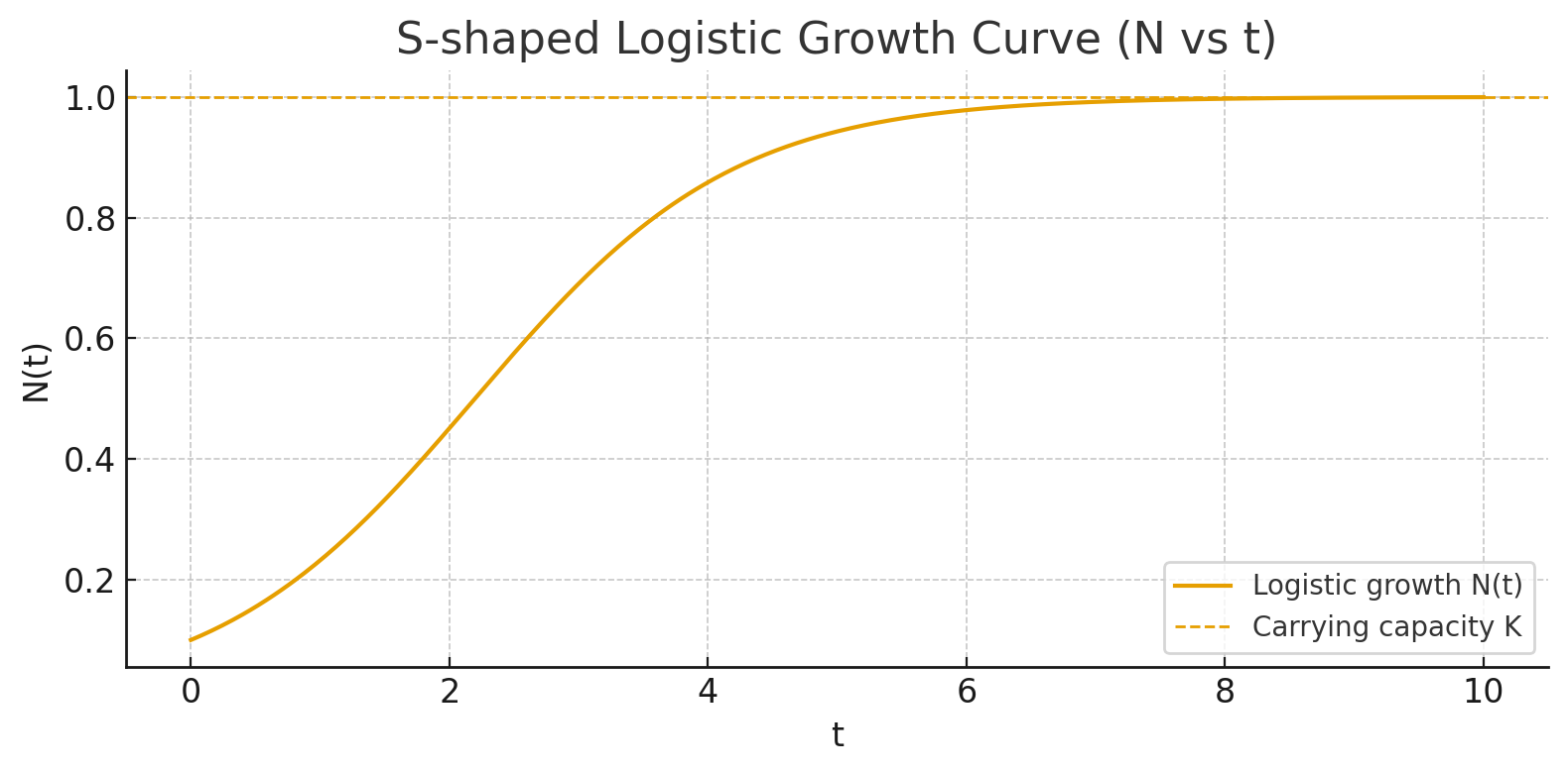
Now, if you follow this flow along the line and integrate it through time, you get the S-shaped logistic curve
In short:
The flow on the line explains why the logistic curve bends the way it does.
The S-shape is the time-domain result of moving along that parabolic flow field.
Linear Stability Analysis
While geometric methods are intuitive, we sometimes need quantitative measures of stability.
That’s where linear stability analysis comes in.
For a fixed point
- If
: stable fixed point - If
: unstable fixed point - If
: indeterminate (requires nonlinear analysis)
The magnitude
Its reciprocal
A Fundamental Limitation: No Oscillations
Here’s a surprising fact: first-order systems cannot oscillate.
Solutions either:
- Approach a fixed point monotonically
- Diverge to infinity
- Remain constant
This is fundamentally topological.
When you flow along a line, you can only move in one direction (or stay still).
You can never return to where you started, so periodic solutions are impossible.
The mechanical analog makes this obvious: imagine a mass in viscous fluid (like honey) attached to a spring.
With enormous damping and negligible inertia, the mass slowly creeps toward equilibrium without any overshoot or oscillation.
The Potential Energy Perspective
There’s an elegant alternative visualization using potential energy.
Define a potential
Now the dynamics can be pictured as a heavily damped particle sliding down the walls of a potential well.
The particle always moves “downhill” toward lower potential:
- Local minima of
→ stable fixed points - Local maxima of
→ unstable fixed points
This perspective is particularly useful in physics and can be extended to more complex systems.
Key Takeaways
- Geometric thinking beats algebraic manipulation for understanding nonlinear systems
- Fixed points dominate the dynamics of first-order systems
- Visual phase portraits reveal qualitative behavior instantly
- First-order systems are fundamentally simple — no oscillations, no chaos
- Multiple perspectives (vector fields, potentials, mechanical analogs) deepen understanding
Looking Ahead
One-dimensional systems are just the beginning.
While they can’t oscillate or exhibit chaos, they provide the essential toolkit for analyzing more complex systems.
The concepts of fixed points, stability, phase portraits, and linearization extend naturally to higher dimensions, where the real excitement begins.
But before tackling those complexities, mastering flows on the line gives you an intuitive foundation that makes everything else easier to understand.
This post summarizes concepts from a course in nonlinear dynamics and chaos, drawing inspiration from Steven H. Strogatz’s Nonlinear Dynamics and Chaos (1994). If you’re interested in learning more, I highly recommend working through similar exercises and experimenting with dynamical systems software to build intuition.